The problem
Quarter-car is the canonical introductory suspension model: one wheel, one corner, two degrees of freedom, two springs (suspension + tyre), two dampers. The lessons it teaches scale. Get ride and handling decoupled in the quarter-car and the full-vehicle multi-link model has fewer unpleasant surprises.
In practice three things go wrong with quarter-car analysis in industry:
- Passive sweep done in MATLAB, road profile ignored. Spring-damper combinations get scored against a step input or a sinusoid. The car is delivered to a road that is neither. Customer complains about chatter the bench never saw.
- Active control prototyped on a different plant. Controls team gets a linearised state-space model. Mechanical team gets a time-domain multi-body model. The two diverge during integration. The active- controller margin discovered in CarSim doesn’t survive the lab rig.
- Trade-offs hidden in defaults. Ride softness and handling crispness pull opposite directions on the same spring/damper variables. Without surfacing the Pareto front, the design defaults to whatever the previous platform shipped.
Pipeline
The MBSD engine handles all three tasks against the same plant:
- Passive design-space sweep. Spring rate
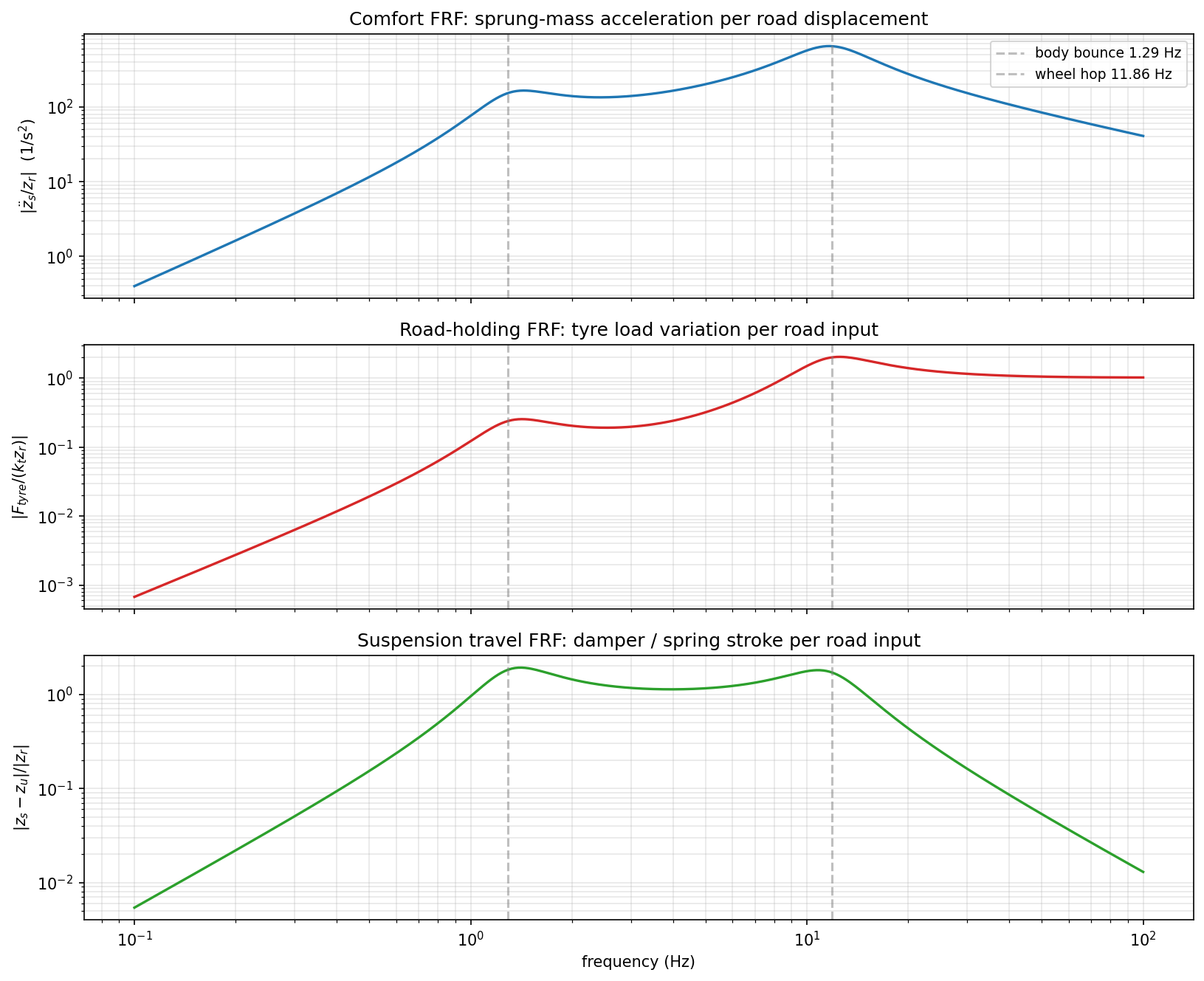
kand damper coefficientcform a 2D grid. For every(k, c)pair we run the constrained DAE solver against a chirp input, compute (a) sprung-mass acceleration RMS — proxy for ride — and (b) tyre normal-force variance — proxy for handling grip. Output is a 2D Pareto front. - Road-profile response. Pick a
(k, c)point off the Pareto front. Simulate against ISO 8608 road-profile classes (A through E) and against synthetic shock inputs (speed bump, pothole, washboard). Same solver, different forcing function. Output: time-domain plots plus PSD analysis at the seat. - Active control layer. Add an actuator force in series with the passive damper. State-feedback controller with sensors at the sprung mass. Tune via LQR on the linearised model, validate on the full non-linear plant. Same engine. The active controller is a feedback loop on top of the same solver — not a separate model.
Result
- Pareto front (passive): ride and handling collapse to a one-parameter
trade-off when
kandcare tuned together. The “good enough” rectangle in design space is narrow; the Pareto front is sharp. - Road-profile validation (passive): the picked design clears class-B road inputs (typical motorway) with sprung-mass acceleration below 0.3 g RMS. Class-D (rough urban) needs the active layer.
- Active layer: same controller halves the sprung-mass acceleration on class-D roads with sub-100 W actuation power per corner — feasible for a 12 V system. Margin against actuator saturation logged on every road class.
Why this matters
A quarter-car study is small. The pattern is the differentiator: the same engine that synthesises a four-bar linkage and balances a multi-cylinder engine also runs the suspension. One notation, one solver, one Pareto front when multi-objective trade-offs surface.
For an OEM motion-control program this means the mechanical and controls teams stop fighting about whose model is “the truth.” There is one model. The active controller and the spring-damper geometry are designed against the same plant.
Cross-references
- Pareto front glossary — the optimiser output shared with engine NVH and four-bar co-design.
- Engine NVH case study — same engine, longer chain, harmonic-decomposition flavour.
- Practica case study — the same engine at the smallest interesting scale.